Table of Contents
Algorithms can modify the layout, the set of selected elements, the size and color of elements, or compute a metric.
As explained in Section 1, “Menus”, algorithms are accessed through the Algorithm menu.
Several algorithms are not installed by default and are avaiable as plugins.
The induced subgraph is the set of selected nodes, and the set of links between selected nodes
Here is an example:
Before:

After:

Kruskal's Algorithm computes a minimum spanning tree of connected graph.
Example:
Before:
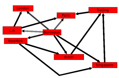
After:
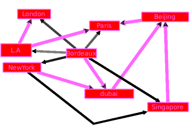
More information: Wikipedia: Minimum spanning tree and Wikipedia: Kruskal's algorithm
Select the loops. A loop is an edge that has the same source and target.
Selects the multiple-edges, also called parallel-edges.
Two edges are parallel iff they both have the same target and same source.
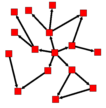
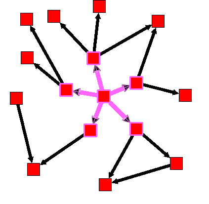
Finds all nodes and edges at distance at most Distance of a set of nodes. It takes three parameters:
Distance: number of edges to follow.Direction: 0 means directed, 1 reverse directed, 2 undirectedStarting nodes: the nodes having this selection property (which msut be boolean) will be used as starting nodes.
In the following example, 'distance' equals 1, 'direction' equals 0, and the starting node is the one in the center.
Before:
After:
Affects colors to the elements, based on one property. In the folling, we take the degree property as an example (which can be computed through Algorithm→Measure→Graph→Degree). The metric mapping algorithm would then compute a color for each node that represents the degree.
Parameters:
Type:- linear: map the full range of degrees (e.g. 0 to 42) to the colorscale, linearly. For instance, if the colorscale is white to black, the degree 21 would be represented as 50% gray.
- uniform: sort the set of existing degrees, then map this set to the colorscale. For instance, if half the nodes have a degree less than 10, the degree ten would be represented as 50% gray.
- enumerated: use this one for properties that have no natural order and a small number of distinct values, like a country name.
Linear/uniform property: If type is linear or uniform, this is the property to be mapped to colors, i.e. the input to be represented visually.Enumerated property: If type is enumerated, this property will be used instead of the above setting.TargetcolorScale
Let's take an example:
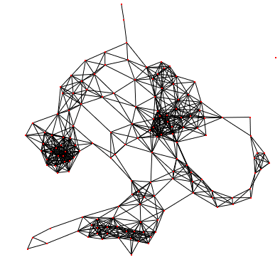
Click Menu Algorithm → Measure → Graph → Degree. The viewMetric property of each node now contains its degree. Now use this property to color the nodes (if menu Options → Map metric is checked, this is done automatically): click menu Algorithm → Color → Color mapping, then OK. After applying the degree algorithm, the graph gets colors!
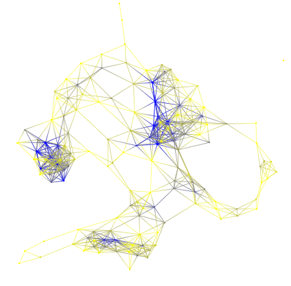
If edges don't have any color, go to View editor → Rendering parameters and check the box "Color interpolation".
Measure algorithms are used to compute different metrics (on edges or nodes). The computed values are assigned to the viewMetric property.
Betweenness measures the centrality of a node within a graph. Nodes that occur on many shortest paths between other nodes have a high betweenness. This algorithm can take a long time to run. More information: Wikipedia: Betweenness.
This algorithm can only be used on simple graphs (i.e. graphs with no loops).
The clustering coefficient measures to which point the saying "friends of friends are friends" applies to the graph at hand. More information: http://en.wikipedia.org/wiki/Clustering_coefficient.
The degree is the number of neighbors. This algorithm takes two parameters:
Type: way to compute the degree of a node:
- In: count only edges pointing to the node.
- Out: count only edges going away from the node.
- InOut: count both.
Metric: if set to none, compute the degree. If set to any other double properties, for instance viewMetric, compute the sum of this property on all adjacent edges.
- Norm
The Eccentricity of a node is the maximum distance between this node and any other one.
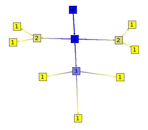
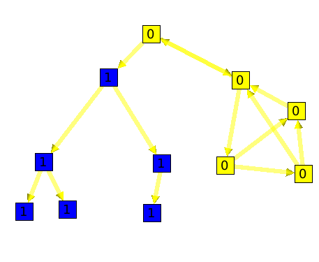
The Strahler algorithm measure branching complexity. It can point out important paths in a graph. Shortly put, on a directed tree, the Strahler number of a node is the max Strahler number of its children. If several children reaches this maximum, then the Strahler number of the parent is one plus this maximum. Here is an example:
This algorithm is a generalization to graphs (i.e. not only trees).
Parameters:
All nodes:If not checked, the algorithm chooses a node (a source node) and applies the algorithm to this node only. If checked, the algorithm is applied to all nodes.Type:
More information: http://en.wikipedia.org/wiki/Strahler_number
A connected graph is biconnected if the removal of any single node and its edges can not disconnect the graph. The biconnected components of a graph are the maximal subsets of nodes such that the removal of a node from a particular component will not disconnect the component. Note that unlike connected components, a node can belong to multiple biconnected components. For example we can use this algorithm on an airlines graph. Such as the one following.
The result is, 3 biconnected components:
1: Paris, New York, L.A, Madrid.
2: Paris, Berlin.
3: Berlin, Moscow, Prague.
The intersection of those 3 biconnected components is Berlin and Paris. Which means that Berlin and Paris are two articulation points of our graph.
A connected component is a maximal connected subgraph. Two nodes are in the same connected component if and only if there exists a path between them.
After running the algorithm, the index of the connected component of a node is saved in its viewMetric property. It is the same for the edges.
for details please visit: Wikipedia:Connected Component Algorithm documentation
The connected tree component algorithm can be useful to find parts of a graph that are trees. Here is an example:
Following is a graph with on the left side, a tree. This graph forms a unique connected component.
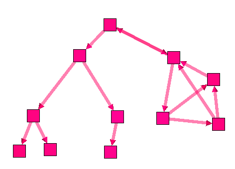
As you can see, the algorithm divided the graph into 2 components.
A directed graph is said to be strongly connected if for every pair of nodes S1 and S2, it exists two edges e1 and e2 such as:
The Source of e1 is S1 and Target is S2 .
The Source of e2 is S2 and Target is S1.
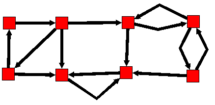
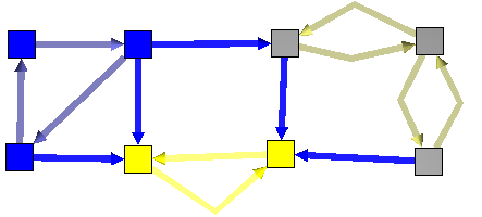
The strongly connected components of a directed graph are its maximal strongly connected subgraphs.
These form a partition of the graph. Here is an example:
Before :
After :
To use the following algorithms the graph has to be acyclic. A graph is acyclic if it contains no cycle.
The dag level algorithm will compute the depth of each node, as on the following example:
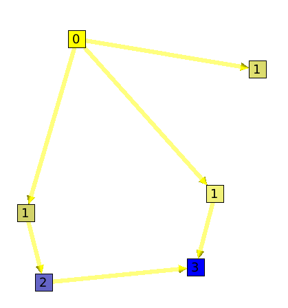
The depth algorithm will compute for each node, the maximum number of edges to follow to find a leaf.
The leaf algorithm will compute for each node its number of leaves.
Here is an example:
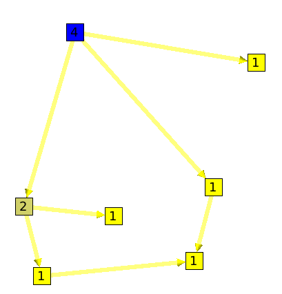
The Node algorithm, will sum for each node the number of its children nodes plus him self. Algorithm documentation
This algorithm will count for each node the number of paths that goes through it.
Here is an example:
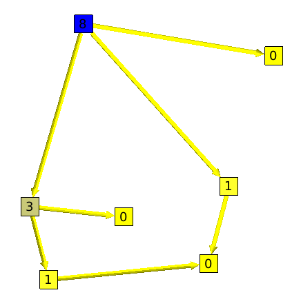
A segment, is a set of nodes that are all on one and only path. The graph showed on the left side of the example is a segment.
The segment algorithm will count, for all nodes, its number of edges without ramification.
Following are two graphs. On the left one you can see that the root "has" 3 edges without ramification. But, on the right graph all nodes (without considering leaves) have only 1 edge without ramification.
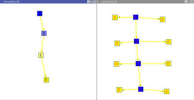
This algorithm can be useful to see how the graph is formed. Indeed, if the root has a small value, it will mean that the graph has a "good" ramification. But if the root has a high value, it will mean that the graph a lot of segments.
Compute the maximum outdegree of the nodes in the subtree induced by each node. To access to the degree of a node it is recommended to use directly the degree function available in each Graph. Algorithm documentation
The "id" algorithm will, for each node and edge, save their id number in their viewMetric Property. For example, if we have a node called Node 9, its id number will be 9. Algorithm documentation
Random will just save a random number (from 0 to 1) in the viewMetric property of each node and edges Algorithm documentation
Warning: Some of the following algorithm have no effect if the option "Force Ratio" is checked.
This algorithm can only be applied to 3-connected graphs. A graph G is said to be 3-connected if there does not exist a set of 2 nodes whose removal disconnects the graph. (Triangle Layout) Algorithm documentation
Create a planar sub-graph with polylines with a good angular resolution which will make the graph clear and easy to read. Algorithm documentation
To represent a tree, a hierarchical layout is the easiest way to understand the tree structure. But this layout has a big weakness when the tree has a lot of nodes: it does not effectively use the space where the tree is displayed. That is why we need different layouts.
The Bubble Tree algorithm can be use to change the layout of a tree. On the new layout, a node will be on the center of a circle, and its children will be on the circle. This new layout has the following properties:
The edges should not cross each other.
The polyline used to draw an edge should have the least possible bends.
The minimal angle between two adjacent edges of a node n should be nearest to 2pi / deg (n). This property will improve the angular resolution.
The order of children of a node should be respected in the final drawing.
Here is an example:
The following graph has the default layout (hierarchical layout). It has a pretty bad angular resolution. Indeed, we do not see the leaves, but only a large black rectangle of edges.
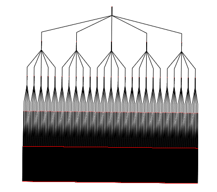
Here is the same tree with a Bubble Tree layout. The angular resolution is much better.
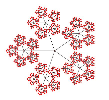
The cone tree is a 3d layout which seen from the top, looks like a bubble tree. It takes two parameters:
node size: size of the node will depend of the metric that you choose. The Algorithm will consider that parameter so that no nodes overlap themselves. This can be useful, if you want a node to be far from the others, just take a new size Metric and give a higher value to that specific node.
Orientation: Vertical / Horizontal
Here is an example of this layout. On the left side you can see a tree with a hierarchical (classic) layout, and, on the right side, the same tree, but with a cone tree layout.
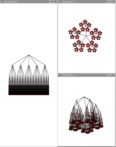
The dendrogram layout is a hierarchical layout on which every leaves are displayed on the same layer.
A dendrogram is a tree diagram frequently used to illustrate the arrangement of the clusters produced by a clustering algorithm. Dendrograms are often used in computational biology to illustrate the clustering of genes.
The algorithm takes 4 parameters:
node size: size of the node will depend of the metric that you choose. The Algorithm will consider that parameter so that no nodes overlap themselves. This can be useful, if you want a node to be far from the others, just take a new size Metric and give a higher value to that specific node.
orientation: up to down, left to right, right to left or down to up.
layer spacing: space between the levels of the Tree.
node spacing: space between sibling nodes.
The hierarchical tree layout looks the same that the dendrogram layout or the improved walker layout but takes an other parameter, "edge length".
node size: size of the node will depend of the metric that you choose. The Algorithm will consider this parameter so that no nodes overlap themselves. This can be useful, if you want a node to be far from the others, just take a new size Metric and give a higher value to that specific node.
edge length: this parameter can take a property of type int, and will be used to place a node on a specific layer. If its value is 1, no thing will happen, but if its value is 2, the node will be placed on the next layer.
orientation: vertical/horizontal;
orthogonal: enables the drawing of the edges, orthogonally bent.
layer spacing: space between the levels of the Tree.
node spacing: space between nodes sibling nodes.
bounding circle: if checked, the estimation of overlapping nodes will be computed with bounding circles instead of bounding rectangles.
The improved walker layout is just a hierarchical layout. Algorithm documentation
The squarified tree map layout, will place nodes in nested rectangles. For example, lets take a tree with a root and two sons, the layout will draw a rectangle for the root containing two other rectangles (its sons). This layout can be very useful for analyzing disks usages.
Here is an example:
Following is the tree a a file system containing 6 file of 1Mb, and several directories.
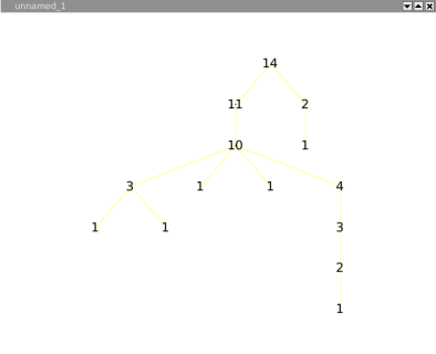
The same graph, with a squarified tree map layout:
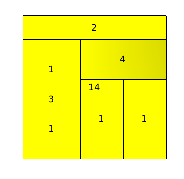
Using the 3D, we can see how the layout is done:
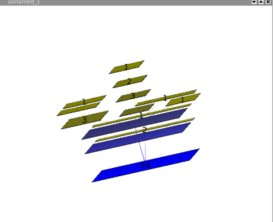
This layout looks like the improved walker, but does not pack the nodes. The result is a nice hierarchical tree in which nodes does not overlap. Algorithm documentation
This layout, is the same as the squarified tree map layout, but the squarified tree map uses shadows to draw the tree. Algorithm documentation
On this layout, nodes of the same layer are placed on a circle whose center is the root. Algorithm documentation
On this layout, every nodes are placed on a circle. Algorithm documentation
This layout groups connected components of the graph so that they do not overlap themselves and that lost space is minimized (packing). It takes 4 parameters:
node size: size of the node will depend of the metric that you choose. The Algorithm will consider that parameter so that no nodes overlap themselves. This can be useful, if you want a node to be far from the others, just take a new size Metric and give a higher value to that specific node.
Rotation.
Coordinates.
Complexity.
Here is an example (left = before, right = after)
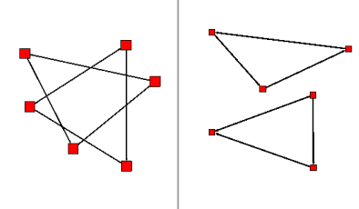
Force Directed layouts will try to place nodes so that, the distance in the graph (metric of the edges) should be the closest to the distance on the drawing.
Warning: The previous property is not 100%.
The GEM layout, unlike the HDE layout, works on all graphs. But it can take a very long computing time if the graph has more than 2000 nodes. Algorithm documentation
This layout, will place the nodes of a graph as if the graph was a tree. Algorithm documentation
The auto sizing algorithm will resize nodes and edges of a graph so that the graph gets easy to read. The size of a node will depend on the number of its sons.
Convolution clustering is an approach to partitioning a graph that gives the user interactive control over how many clusters to create. Tulip calculates a density function based on the chosen metric, displays a convolution of its histogram, and partitions the graph according to the humps in the histogram.
This algorithm will create sub-graphs in which all nodes or all edges (not both at the same time), have the same value. The 'Connected' parameter indicates whether the subgraphs have to be connected or not.
This algorithm will divide the graph in 2 different subgraphs; the first one will contain nodes that have the viewMetric value under than a certain limit, and, the other one, in which nodes will have a the viewMetric value higher than the limit. Then, the algorithm will be re-applied to the subgraph (the one with higher viewMetrics) until the subgraph contains less than 10 nodes. Algorithm documentation
This algorithm will create a metagraph. The metanodes will represent the subgraphs that already exist, and a metaedge will be created between two metanodes if and only if it exist an edge whose source is a node of a subgraph, and the target a node of an other subgraph.
Parameters:
oriented: this parameter indicates whether the graph has to be considered as oriented or not. If it is the case, two metaedges may exist between two metanodes One representing the edges from the nodes of subgraph 1 to the nodes of subgraph 2, the second representing the edges from the nodes of subgraph 2 to the nodes of subgraph 1.
node function: this parameter enables to choose the function used to compute a measure value for a meta-node using the values of its underlying nodes.
edge function: this parameter enables to choose the function used to compute a measure value for a meta-edge using the values of its underlying edges.
meta-node label: this parameter enables to choose the string property used to compute the label of the meta-nodes. An arbitrary underlying node is chosen and its associated value for the given property becomes the meta-node label.This parameter enables to choose the string property to use when naming mete-node.
use name of subgraph: this parameter indicates whether the meta-node label has to be the same as the name of the subgraph it represents. When checked, it supersedes the choice of the previous parameter.
recursive: this parameter indicates whether the algorithm has to be applied along the entire hierarchy of subgraphs.
edge cardinality: this parameter indicates whether the cardinality of the underlying edges of the meta-edges has to be computed or not. If yes, the property edgeCardinality will be created for the quotient graph.
The strength clustering algorithm will recursively create subgraphs that are nested "small-worlds".